2020-05-20
洛谷-P1383 高级打字机 题解Luogu P1383 Advanced Typewriter — Haskell Solution
如果使用 Haskell 语言的话,本题可以使用 containers 包中的 Data.Sequence 秒杀,因为 Seq 本身便是一颗可持久的 FingerTree,用树套树的话,便可以做到一个非常优异的时间/空间复杂度。
惰性求值但是的确是在线算法,可以撤回撤回(返回撤回前的时间点,不知道算不算)。
{-# OPTIONS_GHC -O2 #-} -- 强开O2
import           Control.Monad
import           Data.Functor  (($>))
import           Data.Maybe    (fromJust)
import           Data.Sequence
import           Text.Printf   (printf)

(!) = index -- 强行把函数变成运算符

main :: IO ()
main = do
    n <- readLn :: IO Int -- 读取第一行的整数n,需要手动指定类型,不然会有歧义
    fromList [fromList []] `foldM_'` [1..n] $ \seq _ -> do -- 函数的中缀用法,注意初始的历史记录应该有一个空串
        [[op],c] <- words <$> getLine -- 读取每一行的指令,此处使用了模式匹配(见下文)
        case op of
            'T' -> pure $ (seq!0 |> head c) <| seq  -- 历史记录第0号(即上一次修改的结果)后插入当前字符,然后前插入历史记录
            'U' -> pure $ (seq!read c) <| seq -- 将参数读取为整数(此处无需标明,因为函数有明确的类型限制,编译器将自动推导) 取历史记录的相应项,前插入历史记录
            'Q' -> printf "%c\n" (seq!0!(read c-1))  $> seq -- 将上一次修改的结果的相应位置的字符打印出来,并返回本身的历史记录(($ >)运算符特性)

foldM_' z l f = foldM_ f z l -- 调整参数位置,追求好用
代码十分朴素。
- 空间复杂度: \(O(n\log n)\) ,其中 \(n\) 为总字符数(不是很紧确,但是..能过)
- 每次从后面添加字符,时间复杂度: \(O(1)\)
- 每次打印第 \(i\) 个字符,时间复杂度: \(O(\log (\min (i,n-i)))\) ,其中 \(n\) 为当前字符数, \(i\) 为需要打印的字符位置。
- 每次撤销,时间复杂度: \(O(\log (\min(i,n-i)))\) ,其中 \(n\) 为总修改次数,\(i\) 为撤销步数。
- 总时间复杂度可估算为: \(O(n\log n)\)
如果想看 FingerTree 原理或者希望以此为契机了解一下 Haskell 的话参见后文。也可以参考论文原文。
参考文献:
- Hinze R, Paterson R. Finger trees: a simple general-purpose data structure[J]. Journal of functional programming, 2006, 16(2): 197-217.
- https://hackage.haskell.org/package/fingertree
- https://hackage.haskell.org/package/container
- https://wiki.haskell.org/Functional_dependencies
FingerTree概述
说到可持久化,就得想到 Immutable ,说到 Immutable ,自然而然就是函数式编程语言,说到函数式编程语言,自然而然就是 Haskell ,而说到纯函数式的数据结构,自然而然也绕不开 FingerTree 。
FingerTree 是一种理论上非常通用也非常高效的数据结构,插入头/尾都只需要摊还 \(O(1)\) 的时间,
而对其的“随机”访问只需要 \(O(\log \min(i,n-i))\)
其中 \(i\) 为你访问的下标,所以可以看出访问头/尾其实也是 \(O(1)\) 。
关于它的论文可以戳这里。当然这不是最早的一篇,但我看的就是这篇,才疏学浅没办法在这里列更早的。
但为什么说“理论”上呢,就和斐波那契堆类似,他的常数比较大。(主要因素是Immutable的语言必须维护一个GC来做垃圾回收。)
[更新] 事后我拿
Rust实现了一遍FingerTree,发现其时空消耗均比Haskell大,故可认为并非GC原因。不过也有可能是我写的常数就是大呢(
详见:提交记录
那为什么说“随机”呢?因为完全泛化的 FingerTree 的访问依赖的不是下标,而是一个被称作 \(Measure\) (测度?我也不知道怎么翻译,所以直接拉的原文)的幺半群 (Monoid)。
先解释一下什么是幺半群。幺半群是一个集合 \(X\) 和集合里元素之间一个二元运算 \(\cdot:X\times X\to X\) 的统称(有序对),并要求:
- 二元运算满足结合率,即 \(\forall x,y,z\in X: (x\cdot y)\cdot z = x\cdot (y\cdot z)\)
- 集合 \(X\) 中存在一个单位元,即 \(\exists e:(\forall x: e\cdot x=x\cdot e=x)\)
比如说自然数集 \(\mathbb N\) 与其上的加法 \(+\) 便可以构成一个幺半群(后面我们可以用这条性质做出传统意义上的下标索引)
进一步,我们可以定义两个幺半群的笛卡尔积也是一个幺半群,即对于 \((X,\cdot_1)\) 与 \((Y,\cdot_2)\) , 我们可以定义一个运算 \(\cdot:(X\times Y) \times (X\times Y)\to X\times Y\) ,并使其满足结合率。定义方法如下:
- \((x_1,y_1) \cdot (x_2,y_2)=(x_1\cdot_1 x_2,y_1\cdot_2 y_2)\)
我们可以用这个条件来拓展我们索引方式(比如论文原文里可以看到用 \(\max\) 幺半群实现的最大堆/优先队列)
Haskell基础
首先,用 Haskell 的方式定义一下幺半群(实际上这个标准库有,不需要自己实现)
class Monoid a where
    mempty :: a
    mappend :: a -> a -> a
与常用的C-like语言中的 class 不同,在 Haskell 中,这代表一个类型类,是对类型 a 的一种约束,类似于接口/抽象类一类的概念。
然后是 Foldable ,它代表我们可以在一个类型(其实是一个 Kind ,拿类型生成类型的类型构造子)上按照某种顺序去遍历。类似于 Java 8 中的 reduce 。注意这个其实标准库也有,只是提一嘴。
class Foldable f where
    foldl :: (b -> a -> b) -> b -> f a -> b
    foldr :: (a -> b -> b) -> b -> f a -> b
还需要提一嘴的是 Haskell 最基本的数据结构,链表(实际上还是单端链表,所以只提供最基本的功能)。
data [] a = [] | a:([] a)它意味着一个 \(a\) 类型的链表有两种构造方式,一种是空链表,令一种是一个 \(a\) 类型的元素用 : 运算符拼接一个 \(a\) 类型的链表。(对,中缀构造函数, C++ 是做不到这点的。)
另外还有一个比较常用的 data 被称作 Maybe ,它的定义等价于:
data Maybe a = Nothing | Just a想一想,这个定义是什么意思?
从这里开始就可以看到 Haskell 的一些特性了。Haskell 中的数据结构并非由字段和操作构成,而是由几类数据的组合组合而成。当然它是可以实现上面的俩 class 的。这里我不做过多介绍。
FingerTree 实现(简要复述论文)
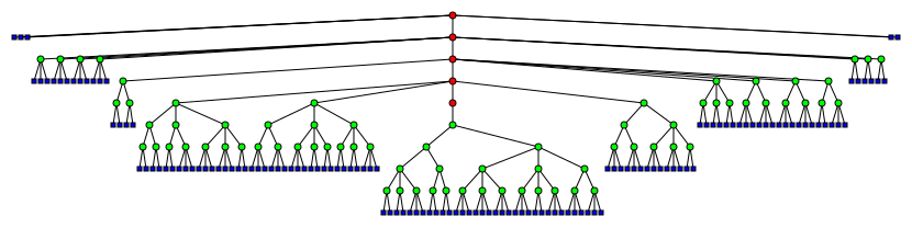
首先是一些基础定义。
-- | Things that can be measured.
class (Monoid v) => Measured v a | a -> v where
    measure :: a -> v

data Node v a = Node2 v a a | Node3 v a a a
data Digit a
    = One a
    | Two a a
    | Three a a a
    | Four a a a a
data FingerTree v a
     = Empty
     | Single a
     | Deep v (Digit a) (FingerTree v (Node v a)) (Digit a)
这里开始出现了最开始提到的 Measured,此处将其抽象为一个可以将某个元素测量出一个 Monoid 的函数。但这个 Monoid 有大用。
此处出现的语法使用了一个 Functional Dependencies 的拓展(可参见 wiki )。大概意思是保证对于一个类型,我只能把它 measure 成一种其他类型,不能 measure 成另一种。也就是说,类型 a 到类型 v 是一个单射。
可以看到这里的 \(v\) 类型变元,这个就是稍后要维护的 Monoid,也是索引数据的依据。
可以看到一个 Node 可能有2-3个元素,保证一个 Digit 有 1-4 个元素。(图中也可以看出,不过引用链接是国外的可能比较卡) Digit 和 Node 也可以相互转化,拼接,但后文不再说明实现。
还有一点值得注意的是,如果当前这一层的 FingerTree 缓存的是 a 类型的话,那么下一层所缓存的就是 Node a 类型了。这也就意味着,下层比上层“厚实”。
自然地,我们可以给 Node 和 Digit 来个 Foldable,但具体部分就不展示了。
那么我们应该如何方便的维护这个 \(v\) 类型的数据呢,答案是换一种方式重写构造函数。
deep ::  (Measured v a) =>
      Digit a -> FingerTree v (Node v a) -> Digit a -> FingerTree v a
 deep pr m sf = Deep ((measure pr `mappend` measure m) `mappend` measure sf) pr m sf
此处的 mappend 是 Haskell 里函数的中缀用法(就是把函数当运算符用)。
此时,我们不需要每次构造树的时候手动维护 \(v\) 类型的数据了,只需要简单把 Deep 替换为 deep 即可。
另外,关于 Measured 本身,我们也可以让 FingerTree 也是 Measured,具体代码如下:
instance (Measured v a) => Measured v (FingerTree v a) where
      measure Empty           =  mempty
      measure (Single x)      =  measure x
      measure (Deep v _ _ _)  =  v
注意到此处使用了 Haskell 被称作模式匹配 (Pattern Match)的特性。(不是模式串匹配啦)把数据结构重新打回了它最开始定义时的样子,并且怎么被构造的就怎么被匹配。(真-打回娘胎)
模式匹配不止可以匹配一层,也可以匹配多层。至于用途嘛..请自行搜索 Haskell 的 20 行红黑树。
可以看到对于 Deep 一类,我们直接使用了其缓存的 \(v\) 类型字段,这样就可以在 \(O(1)\) 时间内得到一颗子树的测度。(如果对单个元素的 measure 也是 \(O(1)\) 的话)
当然 Node 和 Digit 也可以是 Measured,具体实现请自行脑补。
接下来是前插入的定义。
infixr 5 <|
-- | /O(1)/. Add an element to the left end of a sequence.
-- Mnemonic: a triangle with the single element at the pointy end.
(<|) :: Measured v a => a -> FingerTree v a -> FingerTree v a
a <| Empty              =  Single a
a <| Single b           =  deep (One a) Empty (One b)
a <| Deep v (Four b c d e) m sf
    = Deep (measure a `mappend` v) (Two a b) (node3 c d e <| m) sf
a <| Deep v pr m sf     = Deep (measure a `mappend` v) (consDigit a pr) m sf
注意到这里我们自定义了一个运算符,它的优先级是5,并且是右结合的。(不愧是 Haskell,轻易做到了 C++ 做不到的事情。)
consDigit 就是给 pr 前插入一个元素。当然,如果是满的肯定会报错,但是在它之前的模式匹配会避免这一点发生。
类似地还有后插入
infixl 5 .
-- | /O(1)/. Add an element to the right end of a sequence.
-- Mnemonic: a triangle with the single element at the pointy end.
(|>) :: (Measured v a) => FingerTree v a -> a -> FingerTree v a
Empty |> a              =  Single a
Single a |> b           =  deep (One a) Empty (One b)
Deep v pr m (Four a b c d) |> e
    = Deep (v `mappend` measure e) pr (m |> node3 a b c) (Two d e)
Deep v pr m sf |> x     = Deep (v `mappend` measure x) pr m (snocDigit sf x)
可以看到代码基本上和前插入是对称的。(数据结构本身也是对称的,所以这里写作 snocDigit,其中 snoc 正是 cons 的回文)后面还有很多对称的结构,均以左半部分为例。
然后是一个分割原语(当然右侧也是对称的,可以看到又出现了运算符构造子。)
-- | View of the left end of a sequence.
data ViewL s a
     = EmptyL        -- ^ empty sequence
     | a :< s a      -- ^ leftmost element and the rest of the sequence

-- | /O(1)/. Analyse the left end of a sequence.
viewl :: (Measured v a) => FingerTree v a -> ViewL (FingerTree v) a
viewl Empty                     =  EmptyL
viewl (Single x)                =  x :< Empty
viewl (Deep _ (One x) m sf)     =  x :< rotL m sf
viewl (Deep _ pr m sf)          =  lheadDigit pr :< deep (ltailDigit pr) m sf

rotL :: (Measured v a) => FingerTree v (Node v a) -> Digit a -> FingerTree v a
rotL m sf      =   case viewl m of
    EmptyL  ->  digitToTree sf
    a :< m' ->  Deep (measure m `mappend` measure sf) (nodeToDigit a) m' sf
lheadDigit 和 ltailDigit 是指一个 Digit 的最左边元素和剩下的元素,当然如果 Digit 只有一个元素的画 ltail 就会报错,但是前面的模式匹配也避免了这一点。
digitToTree 是一个将 Digit 变为一个 FingerTree 的函数,因为也就常数个元素,所以时间复杂度 \(O(1)\)。
nodeToDigit 也是跟名字异样,将一个 Node(2或3个元素)变成一个 Digit。
case ... of 语法是 Haskell 类似于 C++ 的 switch 语句的地方。不同之处在于其是有返回值的,更像一个多出口的 ?: 运算符。
viewl 函数构造一颗树的左分割,将其切割出最左元素(若没有则用 EmptyL 构造子)。
另外值得注意的是此处的 viewl 和 rotL 是互相调用,也是一种递归哦。
当然其有对称实现 viewr。但不在此赘述。
有了 viewl 之后,我们就可以处理一些 prefix (即 Deep 中第一个 Digit)为空/不存在时对树的构造了
deepL :: (Measured v a) =>
    Maybe (Digit a) -> FingerTree v (Node v a) -> Digit a -> FingerTree v a
deepL Nothing m sf      =   rotL m sf
deepL (Just pr) m sf    =   deep pr m sf
此处的 Nothing 就是指 prefix 不存在的情况,此时需要左旋一波。
当然对于 Just 的情况就直接调用上面的deep了。
那么什么情况下左边/右边为空呢?当然是做分割的时候了。
那么终于,要迎来最后的部分了,搜索,与分割。
data Split t a = Split t a t
data SearchResult v a
    = Position (FingerTree v a) a (FingerTree v a)
        -- ^ A tree opened at a particular element: the prefix to the
       -- left, the element, and the suffix to the right.
   | OnLeft
       -- ^ A position to the left of the sequence, indicating that the
       -- predicate is 'True' at both ends.
   | OnRight
       -- ^ A position to the right of the sequence, indicating that the
       -- predicate is 'False' at both ends.
   | Nowhere
       -- ^ No position in the tree, returned if the predicate is 'True'
       -- at the left end and 'False' at the right end.  This will not
       -- occur if the predicate in monotonic on the tree.

search :: (Measured v a) =>
    (v -> v -> Bool) -> FingerTree v a -> SearchResult v a
search p t
  | p_left && p_right = OnLeft
  | not p_left && p_right = case searchTree p mempty t mempty of
         Split l x r -> Position l x r
  | not p_left && not p_right = OnRight
  | otherwise = Nowhere
   where
     p_left = p mempty vt
     p_right = p vt mempty
     vt = measure t

searchTree :: (Measured v a) =>
     (v -> v -> Bool) -> v -> FingerTree v a -> v -> Split (FingerTree v a) a
searchTree _ _ Empty _ = illegal_argument "searchTree"
searchTree _ _ (Single x) _ = Split Empty x Empty
searchTree p vl (Deep _ pr m sf) vr
  | p vlp vmsr  =  let  Split l x r     =  searchDigit p vl pr vmsr
                   in   Split (maybe Empty digitToTree l) x (deepL r m sf)
  | p vlpm vsr  =  let  Split ml xs mr  =  searchTree p vlp m vsr
                        Split l x r     =  searchNode p (vlp `mappend` measure ml)       xs (measure mr `mappend` vsr)
                   in   Split (deepR pr  ml l) x (deepL r mr sf)
  | otherwise   =  let  Split l x r     =  searchDigit p vlpm sf vr
                   in   Split (deepR pr  m  l) x (maybe Empty digitToTree r)
  where
    vlp     =  vl `mappend` measure pr
    vlpm    =  vlp `mappend` vm
    vmsr    =  vm `mappend` vsr
    vsr     =  measure sf `mappend` vr
    vm      =  measure m
此处只列出了 searchTree 这一子函数,且十分冗长,其实 searchNode 和 searchDigit 也类似,本质上就是为了找到第一个使得对于输入的函数,在值左边的分割为假,右边的为真。一步步细化下去而已。
maybe 函数的类型是 b -> (a -> b) -> Maybe a -> b,看类型签名基本可以猜到功能。所以也不细说。
这里可以看到 where 从句。where 从句和常量定义很像,但却是后置的,而且具有惰性求值的特征(对,自带Lazy,而且实际上如果不做额外标注,整个 Haskell 程序都是惰性求值的)。
到这一步为止,我们只差将原本用于索引的下标整成 Monoid 就好了,并且其和任意类型均可以构成 Measured(因为单个元素大小都是1)
newtype Size = Size Int
newtype Elem a = Elem a
instance Monoid Size where
	mempty = Size 0
	mappend (Size a) (Size b) = Size (a+b)
instance Measured Size (Elem a) where
	measure _ = Size 1
这里注意,由于我们之前使用了 Functional Dependencies,所以我们需要新建一个类型作为容器来容纳我们的类型。所以此处使用了不会导致额外开销的 newtype 关键字替代 data(在当前环境下,二者语义一致)
接下来就可以实现 Seq 了,具体可以参考 container 包的源代码或者论文原文。
If you’re using Haskell, this problem can be solved trivially with Data.Sequence from the containers package, because Seq itself is a persistent FingerTree — a tree-of-trees approach gives excellent time and space complexity.
Lazy evaluation keeps it an online algorithm. It can even undo undos (return to the state before the undo).
{-# OPTIONS_GHC -O2 #-}
import           Control.Monad
import           Data.Functor  (($>))
import           Data.Maybe    (fromJust)
import           Data.Sequence
import           Text.Printf   (printf)

(!) = index

main :: IO ()
main = do
    n <- readLn :: IO Int
    fromList [fromList []] `foldM_'` [1..n] $ \seq _ -> do
        [[op],c] <- words <$> getLine
        case op of
            'T' -> pure $ (seq!0 |> head c) <| seq
            'U' -> pure $ (seq!read c) <| seq
            'Q' -> printf "%c\n" (seq!0!(read c-1))  $> seq

foldM_' z l f = foldM_ f z l
The code is straightforward.
- Space complexity: \(O(n\log n)\), where \(n\) is the total number of characters.
- Appending a character: \(O(1)\).
- Printing the \(i\)-th character: \(O(\log(\min(i,n-i)))\).
- Undoing: \(O(\log(\min(i,n-i)))\), where \(n\) is the total number of modifications and \(i\) the undo steps.
- Overall: \(O(n\log n)\).
If you’re interested in the FingerTree internals or want to use this as an opportunity to learn Haskell, see below. The original paper is also a good reference.
References:
- Hinze R, Paterson R. Finger trees: a simple general-purpose data structure[J]. Journal of functional programming, 2006, 16(2): 197-217.
- https://hackage.haskell.org/package/fingertree
- https://hackage.haskell.org/package/container
- https://wiki.haskell.org/Functional_dependencies
FingerTree Overview
When it comes to persistence, you think Immutable. When you think Immutable, you think functional programming languages. When you think functional programming, you think Haskell. And when you think purely functional data structures, you can’t avoid FingerTree.
FingerTree is a theoretically very general and efficient data structure. Inserting at either end takes amortized \(O(1)\), and “random” access takes \(O(\log\min(i,n-i))\).
\(i\) is the index, so accessing the ends is indeed \(O(1)\).
The paper can be found here. This isn’t the earliest paper, but it’s the one I read.
Why “theoretically”? Like Fibonacci heaps, the constant factor is large. (The main factor is that immutable languages need a GC for garbage collection.)
[Update] I later implemented FingerTree in Rust and found its time and memory consumption both larger than Haskell’s, so the overhead probably isn’t due to GC.
Though it could just be my poor constant factors.
See: submission record
Why “random”? Because fully generalized FingerTree access depends not on indices but on a Monoid called a Measure.
A monoid is a set \(X\) with a binary operation \(\cdot:X\times X\to X\) satisfying:
- Associativity: \(\forall x,y,z\in X: (x\cdot y)\cdot z = x\cdot (y\cdot z)\)
- Identity: \(\exists e:(\forall x: e\cdot x=x\cdot e=x)\)
For example, \(\mathbb N\) with addition \(+\) forms a monoid (which gives us traditional indexing).
The Cartesian product of two monoids is also a monoid. If \((X,\cdot_1)\) and \((Y,\cdot_2)\) are monoids, define \(\cdot:(X\times Y)\times(X\times Y)\to X\times Y\) as:
- \((x_1,y_1) \cdot (x_2,y_2)=(x_1\cdot_1 x_2,y_1\cdot_2 y_2)\)
This extends our indexing capabilities (e.g., the paper uses a \(\max\) monoid to implement max-heap/priority queues).
Haskell Basics
First, define a monoid in Haskell (the standard library provides this):
class Monoid a where
    mempty :: a
    mappend :: a -> a -> a
Unlike C-like languages’ class, in Haskell this is a type class — a constraint on type a, similar to an interface or abstract class.
Next, Foldable represents the ability to traverse a type (actually a kind — a type constructor that produces types) in some order. Similar to reduce in Java 8. This is also in the standard library.
class Foldable f where
    foldl :: (b -> a -> b) -> b -> f a -> b
    foldr :: (a -> b -> b) -> b -> f a -> b
Also worth mentioning is Haskell’s most basic data structure, the list (a singly-linked list with basic operations):
data [] a = [] | a:([] a)A list of type a is either empty or an a element consed with another list using the : operator. (An infix constructor — C++ can’t do this.)
Another common data type is Maybe, equivalent to:
data Maybe a = Nothing | Just aThis is where Haskell’s character starts to show. Data structures in Haskell are built not from fields and operations, but from combinations of constructors. They can implement the two type classes above. I won’t go into detail here.
FingerTree Implementation (Brief Summary of the Paper)
Basic definitions:
-- | Things that can be measured.
class (Monoid v) => Measured v a | a -> v where
    measure :: a -> v

data Node v a = Node2 v a a | Node3 v a a a
data Digit a
    = One a
    | Two a a
    | Three a a a
    | Four a a a a
data FingerTree v a
     = Empty
     | Single a
     | Deep v (Digit a) (FingerTree v (Node v a)) (Digit a)
Here we encounter the Measured type class mentioned earlier. It abstracts a function that measures an element into a Monoid. This monoid has important uses.
The syntax uses a Functional Dependencies extension (see wiki). It guarantees that a given type maps to exactly one measure type — a type a to type v is an injection.
The type variable \(v\) is the Monoid that will be maintained and used for indexing.
A Node has 2-3 elements; a Digit has 1-4 elements (as shown in the diagram). Digits and Nodes can be interconverted and concatenated.
Notably, if the current layer of FingerTree caches type a, the next layer caches type Node v a. This means each lower layer is “thicker” than the one above.
Naturally, we can make Node and Digit instances of Foldable, but I won’t show that here.
How to conveniently maintain the $v` value? Write a smart constructor:
deep :: (Measured v a) =>
      Digit a -> FingerTree v (Node v a) -> Digit a -> FingerTree v a
 deep pr m sf = Deep ((measure pr `mappend` measure m) `mappend` measure sf) pr m sf
Now we don’t need to maintain \(v\) manually — just replace Deep with deep.
FingerTree itself can also be Measured:
instance (Measured v a) => Measured v (FingerTree v a) where
      measure Empty           =  mempty
      measure (Single x)      =  measure x
      measure (Deep v _ _ _)  =  v
This uses Haskell’s pattern matching — the data structure is deconstructed the same way it was constructed.
Pattern matching works on multiple levels. See Haskell’s 20-line red-black tree for an example.
For Deep, we directly use the cached \(v\) field, giving \(O(1)\) access to a subtree’s measure (if measure on a single element is also \(O(1)\)).
Node and Digit can also be Measured — the implementation is left as an exercise.
Next, the definition of cons (left insertion):
infixr 5 <|
-- | /O(1)/. Add an element to the left end of a sequence.
-- Mnemonic: a triangle with the single element at the pointy end.
(<|) :: Measured v a => a -> FingerTree v a -> FingerTree v a
a <| Empty              =  Single a
a <| Single b           =  deep (One a) Empty (One b)
a <| Deep v (Four b c d e) m sf
    = Deep (measure a `mappend` v) (Two a b) (node3 c d e <| m) sf
a <| Deep v pr m sf     = Deep (measure a `mappend` v) (consDigit a pr) m sf
We define a custom operator with precedence 5, right-associative.
consDigit prepends an element to pr. If it’s full, it would error, but the pattern match above prevents that.
Similarly for snoc (right insertion):
infixl 5 .>
-- | /O(1)/. Add an element to the right end of a sequence.
-- Mnemonic: a triangle with the single element at the pointy end.
(|>) :: (Measured v a) => FingerTree v a -> a -> FingerTree v a
Empty |> a              =  Single a
Single a |> b           =  deep (One a) Empty (One b)
Deep v pr m (Four a b c d) |> e
    = Deep (v `mappend` measure e) pr (m |> node3 a b c) (Two d e)
Deep v pr m sf |> x     = Deep (v `mappend` measure x) pr m (snocDigit sf x)
The code is symmetric to cons.
A splitting primitive (right side is symmetric):
-- | View of the left end of a sequence.
data ViewL s a
     = EmptyL        -- ^ empty sequence
     | a :< s a      -- ^ leftmost element and the rest of the sequence

-- | /O(1)/. Analyse the left end of a sequence.
viewl :: (Measured v a) => FingerTree v a -> ViewL (FingerTree v) a
viewl Empty                     =  EmptyL
viewl (Single x)                =  x :< Empty
viewl (Deep _ (One x) m sf)     =  x :< rotL m sf
viewl (Deep _ pr m sf)          =  lheadDigit pr :< deep (ltailDigit pr) m sf

rotL :: (Measured v a) => FingerTree v (Node v a) -> Digit a -> FingerTree v a
rotL m sf      =   case viewl m of
    EmptyL  ->  digitToTree sf
    a :< m' ->  Deep (measure m `mappend` measure sf) (nodeToDigit a) m' sf
lheadDigit and ltailDigit get the leftmost element of a Digit and the rest. If the Digit has only one element, ltailDigit would error, but the pattern match prevents that.
digitToTree converts a Digit to a FingerTree (constant number of elements, so \(O(1)\)).
nodeToDigit converts a Node (2 or 3 elements) to a Digit.
case ... of is Haskell’s analog of C++’s switch, but it has a return value — more like a multi-branch ?: operator.
viewl constructs a left view of the tree, extracting the leftmost element (or EmptyL if none).
Note that viewl and rotL are mutually recursive.
There’s a symmetric viewr implementation.
With viewl, we can handle the case where the prefix (the first Digit in Deep) is empty/missing:
deepL :: (Measured v a) =>
    Maybe (Digit a) -> FingerTree v (Node v a) -> Digit a -> FingerTree v a
deepL Nothing m sf      =   rotL m sf
deepL (Just pr) m sf    =   deep pr m sf
Nothing means the prefix doesn’t exist — need a left rotation. Just calls deep directly.
When would the left/right be empty? During splitting.
Finally, search and split:
data Split t a = Split t a t
data SearchResult v a
    = Position (FingerTree v a) a (FingerTree v a)
        -- ^ A tree opened at a particular element: the prefix to the
       -- left, the element, and the suffix to the right.
   | OnLeft
       -- ^ A position to the left of the sequence, indicating that the
       -- predicate is 'True' at both ends.
   | OnRight
       -- ^ A position to the right of the sequence, indicating that the
       -- predicate is 'False' at both ends.
   | Nowhere
       -- ^ No position in the tree, returned if the predicate is 'True'
       -- at the left end and 'False' at the right end.  This will not
       -- occur if the predicate in monotonic on the tree.

search :: (Measured v a) =>
    (v -> v -> Bool) -> FingerTree v a -> SearchResult v a
search p t
  | p_left && p_right = OnLeft
  | not p_left && p_right = case searchTree p mempty t mempty of
         Split l x r -> Position l x r
  | not p_left && not p_right = OnRight
  | otherwise = Nowhere
   where
     p_left = p mempty vt
     p_right = p vt mempty
     vt = measure t

searchTree :: (Measured v a) =>
     (v -> v -> Bool) -> v -> FingerTree v a -> v -> Split (FingerTree v a) a
searchTree _ _ Empty _ = illegal_argument "searchTree"
searchTree _ _ (Single x) _ = Split Empty x Empty
searchTree p vl (Deep _ pr m sf) vr
  | p vlp vmsr  =  let  Split l x r     =  searchDigit p vl pr vmsr
                   in   Split (maybe Empty digitToTree l) x (deepL r m sf)
  | p vlpm vsr  =  let  Split ml xs mr  =  searchTree p vlp m vsr
                        Split l x r     =  searchNode p (vlp `mappend` measure ml) xs (measure mr `mappend` vsr)
                   in   Split (deepR pr ml l) x (deepL r mr sf)
  | otherwise   =  let  Split l x r     =  searchDigit p vlpm sf vr
                   in   Split (deepR pr m l) x (maybe Empty digitToTree r)
  where
    vlp     =  vl `mappend` measure pr
    vlpm    =  vlp `mappend` vm
    vmsr    =  vm `mappend` vsr
    vsr     =  measure sf `mappend` vr
    vm      =  measure m
I’ve only shown searchTree here. searchNode and searchDigit are similar — they find the first position where the predicate returns False on the left side and True on the right side, then recurse down.
The maybe function has type b -> (a -> b) -> Maybe a -> b. Its signature reveals its purpose.
Note the where clause. It’s like a constant definition, but post-posed and lazy. (Without explicit annotation, the entire Haskell program is lazy.)
We’re now only missing one piece: indexing with a Monoid that can beMeasured for any type (since each element counts as 1):
newtype Size = Size Int
newtype Elem a = Elem a
instance Monoid Size where
    mempty = Size 0
    mappend (Size a) (Size b) = Size (a+b)
instance Measured Size (Elem a) where
    measure _ = Size 1
Note: since we used Functional Dependencies, we need a new wrapper type. We use newtype instead of data (both cost nothing at runtime in this context).
From here, Seq can be implemented — see the containers package source or the original paper for details.